Primary target surface
These rendering routes are generated from canonical source. Native-WebGPU acceptance remains separate from entrypoint availability.
Solve bounded and coastal water in Three.js WebGPU/TSL. Use for parametric waves, local heightfields, bathymetric wave transport, wet/dry shallow water, two-way body coupling, external free-surface presentation, or water optics and offshore handoffs.
These rendering routes are generated from canonical source. Native-WebGPU acceptance remains separate from entrypoint availability.
This skill contributes to the following cross-skill owner graphs.
Source hashes, claim verdicts, promoted same-lab media, fixed routes, exact tier contracts, and current limitations.
Bounded water couples a compute heightfield with physically-grounded shading. The simulation integrates the damped wave equation on a storage-texture ping-pong:
$$\frac{\partial^2 h}{\partial t^2} = c^2 \nabla^2 h - \beta\,\frac{\partial h}{\partial t}$$Underwater light follows Beer–Lambert absorption along the refracted path length $d$, per RGB channel (red dies first):
$$L(d) = L_0\, e^{-\sigma_a d}, \qquad \sigma_a = (\sigma_r, \sigma_g, \sigma_b)$$Caustics come from the differential-area ratio of a refracted beam — brightness is the inverse Jacobian of the ray-footprint map, and Fresnel splits reflection/refraction by angle (Schlick approximation):
$$I_c \propto \left|\det \frac{\partial \mathbf x_{floor}}{\partial \mathbf x_{surface}}\right|^{-1}, \qquad F(\theta) = F_0 + (1-F_0)(1-\cos\theta)^5$$Only schema-v2 labs with accepted runtime and evidence contracts appear here. Other source directories remain visible through the demo registry without being promoted to runnable proof.
Every image identifies what it proves. Page screenshots demonstrate the published presentation only; generated inputs demonstrate asset channels only; rendering acceptance still requires same-lab readback and a schema-v2 bundle.
0 published imagesThe complete SKILL.md as loaded by agents, rendered verbatim.
Select the least complex water representation that owns the requested observable, then derive displacement, derivatives, foam, wetness, and optical transport from that state.
| Required observable | Representation | Invalid when |
|---|---|---|
| Static surface and bathymetry; only bottom visibility, refraction, attenuation, or caustics matter | Static bathymetry plus optical transport | Surface motion, waterline motion, or interaction is required |
| Prescribed coast-following crests; no flow or interaction claim | Coast SDF plus prescribed shoreline phase | Diffraction, run-up, bulk flow, or changing wet/dry topology matters |
| Few coherent waves; no local disturbance | Parametric displaced surface | Broad stochastic bands or dense interaction dominate |
| Bounded weak waves and local impulses | Linear heightfield | Breaking, bulk flow, or wet/dry topology matters |
| Fixed bathymetry; phase-averaged shoaling/refraction | Wave action or rays | Diffraction, interference, or instantaneous crest parity matters |
| Fixed bathymetry; linear diffraction/interference | Frequency-domain mild slope | Breaking, run-up, moving bed, or live broad spectra matter |
| Long waves over permanently wet variable depth | Linear elevation/discharge shallow water | Wet/dry fronts, bores, or finite-amplitude flow matter |
| Run-up, bores, depth-averaged wakes, or changing wet topology | Positivity-preserving nonlinear shallow water | Dispersive or three-dimensional breaking is required |
| Overturning, entrained air, jets, or three-dimensional vortices | External free-surface/particle/VOF solver | A single-valued or depth-averaged model is sufficient |
| Body motion affects water and water reaction affects the body | Selected water solver plus the two-way coupling branch | One-way visual following or a prescribed wake is sufficient |
Route broad homogeneous wind sea or swell to $threejs-spectral-ocean. Normal-
only detail is a display optimization, not another physical owner.
Record domain size, smallest resolved wavelength, interaction radius, bathymetric variation, phase/error tolerance, conservation needs, wet/dry topology, and sustained budget. Hybridize only across an explicit spatial or frequency handoff.
Complete when: every required observable has exactly one valid owner and every rejected representation has a stated validity or measured cost reason.
Use metres and seconds in a stable physics frame:
z_b(x,z) = upward-positive bed elevation
eta(x,z,t) = free-surface elevation
h = max(eta-z_b,0)

phi > 0 on land
phi = 0 at the authored still-water coast
phi < 0 in water.
Declare the water datum, gravity, bed and coast-distance sources, valid mask, cell footprint, reconstruction/filter, boundary labels, obstacle representation, current, and clock. Horizontal coast distance is not vertical water depth.
Assign exactly one owner to water state, geometry, offshore forcing, foam, exposed-bed wetness, caustics, opaque refraction inputs, and final output. Every boundary is periodic, reflecting/wall, absorbing/radiation, prescribed inflow, or outflow with a named mathematical treatment.
For each water boundary, declare producer, consumer, and state owner; units and
stable physics frame/origin; sample instant or application interval, clock,
cadence, and sample phase; support/filter; validity, staleness, and error; and
state/resource versions. Distinguish rates from interval-integrated mass,
momentum, or energy. Name forcing, reaction, geometry, and presentation
ownership and their order. A clock discontinuity, rebase, representation or
owner change, or incompatible version resets every dependent solver, foam,
wetness, query, and temporal state. Invoke $threejs-choose-skills when a
multi-system route still needs ownership selection.
Complete when: bed, coast, datum, state, boundary, clock, and output
ownership agree at every sample; the SDF zero contour and z_b=eta_0 contour
meet their declared gate.
Read only the linked heading span: start at the heading and stop before the next heading at the same or higher level.
| Selected representation | Required reference spans |
|---|---|
| Static surface and bathymetry | Domain data and invariants, then the required optical spans below |
| Parametric displaced surface | Exact parametric waves and Physics-horizontal queries |
| Bounded linear heightfield | Bounded linear heightfield |
| Prescribed coast-following phase | Domain data and invariants and Prescribed shoreline phase |
| Wave action or rays | Domain data and invariants and Depth-aware wave action and rays |
| Frequency-domain mild slope | Domain data and invariants and Mild-slope branch |
| Fixed-wet linear shallow water | Domain data and invariants and Fixed-wet linear shallow water |
| Nonlinear wet/dry shallow water | Domain data and invariants and Nonlinear shallow water with wet/dry fronts |
| External solver | Use the External solver adapter contract below; load only shared spans needed by its published channels |
Load these additional spans only when the named concern is selected:
After a surface/optics branch, apply the matching bullets in surface acceptance. After a coastal branch, apply the matching bullets in coastal acceptance.
Evaluate one displacement map, both analytic tangents, the horizontal Jacobian, and the upward cross-product normal. Physics-horizontal queries invert the horizontal map.
Branch complete when: parameter and physics-horizontal samples have unambiguous semantics; analytic tangents/normals match finite differences; the minimum Jacobian is positive or every fold is classified invalid; and query residuals meet their gate.
Use ping-ponged height/vertical-velocity state, fixed dt, dimensioned
sources, an explicit boundary condition, and this dispatch order:
event gather -> propagate -> swap -> derivatives -> optical auxiliaries.
Before accepting this branch, import the
bounded-heightfield dispersion comparator
and call boundedHeightfieldDispersion() with the selected c, dt, dx,
dz, kx, and kz. It predicts the undamped (gamma=0) discrete phase;
compare that prediction with the measured analytic-mode phase. Measure
amplitude error independently for the actual damping and source configuration.
Branch complete when: the CFL margin is positive; analytic-mode phase and amplitude errors, boundary reflection, mean drift, precision error, and finite-value scan pass; overlapping events have no write race; and every consumer reads derivatives from the new state.
Derive crest phase from coast distance or a converged eikonal travel-time field. The phase branch owns crest placement and a prescribed wash mask only; it makes no flow, momentum, or wave-energy claim.
Branch complete when: crest direction, spacing, and speed; coastwise continuity; eikonal residual and unreachable classification; medial-axis coast ownership; and fragment-footprint filtering all pass their gates, with the no-flow/no-energy claim explicit.
Transport dimensioned action/energy by frequency and direction. Keep current, intrinsic frequency, group velocity, quadrature, dissipation, and a separately owned display phase explicit. Rays make no diffraction/interference claim.
Branch complete when: dispersion/group velocity, phase-loop or curl, action/energy balance, shoaling/refraction, regularization, and handoff reflection pass over the represented band.
Solve complex phase/amplitude for fixed, slowly varying bathymetry with radiation/open boundaries. Prefer an offline solution when sources and bathymetry are stationary.
Branch complete when: manufactured or independent-reference convergence, phase/amplitude interpolation, boundary reflection, and stored-field invalidation pass.
Evolve surface perturbation and depth-integrated discharge with compatible discrete divergence/gradient or one finite-volume flux.
Branch complete when: permanently wet state is enforced; mass and declared energy behavior close; dispersion and boundary reflection pass; and no wet/dry, bore, or finite-amplitude claim is made.
Evolve conservative depth and momentum with one canonical face flux, well-balanced bathymetry, positivity-preserving update, dry-cell division policy, fixed stable step, and conservative source accounting.
Branch complete when: depth stays nonnegative without unreported clamping; lake at rest remains stationary; mass closes against boundary/source fluxes; dry cells stay finite; shoreline/run-up and grid/timestep/dry-threshold convergence pass; and boundary reflection is within gate.
Consume its versioned surface, velocity, wet/dry, material, and presentation state through an explicit adapter. Keep external process/queue/fence latency and unavailable channels visible.
Branch complete when: units, frame, clock, interpolation, error, lifecycle, failure/recovery, and presentation ownership are proven; the render frame does not synchronously read back or advance the external solve.
When body motion must affect water and water must react on the body, use one declared coupling interval:
predict body state
-> sample the same previous/current water bracket at body support points
-> scatter displacement or impulse to water conservatively
-> advance water once
-> reduce reaction force, torque, and interface work over the same support
-> correct body state
-> commit both versions together.
Use one physics frame, units, sample identity, and support/Jacobian convention. Keep collision and render LOD out of the coupling support. Classify the method as explicit loose coupling or bounded residual iteration; strong added-mass or stiff feedback requires the iterative branch or an external coupled solver.
Branch complete when: equal-and-opposite impulse, force, torque, displaced volume, and interface-work residuals meet their gates; stationary buoyancy, translation/rotation, grid/timestep, and iteration controls converge; and no render-frame readback advances or corrects either state.
Geometry, tangents, normal, velocity, shadows, foam source, refraction, and temporal consumers derive from the selected state version. A handoff has one geometry owner at every location. Coherent surfaces use matched amplitude and differentiate the blend, including weight gradients; power windows apply only to independent or orthogonal bands.
Build one foam source from the strongest represented cause: modeled breaking loss, calibrated shock/entropy loss, exact compression/Jacobian, or prescribed crest arrival. Store either transported coverage or conserved areal density and use its matching equation. One dissipation partition drives one history.
Exactly one exposed-bed receiver owns wetness. Inundation or a declared prescribed wash mask sets it wet; drying is timestep-correct. Wetness changes receiver material response, not water mass or shoreline geometry.
For sparse coastal execution, activate from causal influence and interaction support rather than visibility alone. Fill halos and boundaries before whole-tile stencils; preserve one face flux across neighbors; account for activation/deactivation state and error.
Complete when: one state version explains every geometric and optical consumer, foam and wetness each have one owner and reset rule, sparse inactive regions have an explicit model, and no displayed seam has two surfaces.
The opaque color/depth input excludes water. Reconstruct and validate the refracted ray before using its length. Classify the incident side, use exact dielectric Fresnel near total internal reflection, and apply Beer-Lambert extinction in metres:
sigma_t = sigma_a + sigma_s
T = exp(-sigma_t pathLengthMeters)

L_water = F L_reflection
        + (1-F) [T L_background + (1-T) omega_0 L_source].
Foam replaces a bounded fraction of this response. A specular BRDF owns sun glint unless another explicitly budgeted lobe replaces it.
Caustics deposit surface-cell power in receiver space using the determinant of the receiver map. Track invalid/TIR samples, power before and after deposition, regularization, filtering, and clamp.
Complete when: Fresnel/TIR classification, refracted-ray residual, path-length validity, absorption/scattering partition, caustic receiver placement, energy ledger, and final/no-optics/no-caustics/no-foam views pass.
Run await renderer.init() and require
renderer.backend.isWebGPUBackend === true before allocating or submitting
compute/storage work. Simulation textures use NoColorSpace, explicit
precision, no generated mips, and integer loads for stencils. Each whole-grid
producer/consumer dependency crosses a dispatch boundary.
renderer.computeAsync(...) is initialization-safe; its resolved promise is
not GPU-completion evidence. Keep simulation resolution independent of
viewport resolution.
Render with one scene pass, one RenderPipeline, and one output transform. If
renderOutput(...) owns conversion, set
pipeline.outputColorTransform = false. After replacing
pipeline.outputNode, set pipeline.needsUpdate = true.
Presentation consumes immutable previous/current state with stable identity.
Resize, representation, cadence, active-domain, datum, origin, source, and
solver-version changes migrate compatible state or reset every dependent
history. Dispose resources and listeners with their owner.
Complete when: the initialized native-WebGPU backend/capabilities, dispatch and allocation inventory, peak live bytes, precision comparison, warm sustained timings, and rebuild/dispose plateau are recorded; no frame-critical readback or double output transform remains.
Inspect the applicable diagnostics, not only the final image:
Complete when: every selected branch criterion passes, every omitted phenomenon is outside the claim, every handoff has one producer and consumer, every resource has an owner and reset/dispose rule, and one causal water state reaches one final output transform.
Preserved concept proxies and generated-asset previews. They are excluded from primary completion counts and link to the canonical lab through the schema-v2 registry.